Ambient noise consists of various components, which are detailed in the following discussion. Four primary noise sources are examined more closely. Specifically, ship noise, as represented by the Wenz curves, and wind-driven surface noise are presented both as digitized data points and through mathematical equations. To provide a comprehensive overview of the basic noise spectrum, equations for noise resulting from ocean turbulence and thermally driven microscopic motion are also included. However, this overview does not account for noise generated by rain or seismic activities, as these sources are typically shorter in duration and highly variable in nature.
Ship noise
Noise from shipping is the main cause of ambient noise as frequencies between some tens of Hz and 1 kHz. Noise intensity from a ship is highly variable and depends heavily on the type of ship, its propulsion system and its speed. While noise from close-by ships may be considered transitory, noise from distant shipping is more consistent and may be described by the following empirical model:
$$ NL_{ship}(w,f) = 20+12w+20\log(f)-30\log(f^2+(15+4w)/10^4) $$
with \(w=[0,1,2]\) indicating light,medium, and heavy shipping and frequency \(f\) in kHz
Wind driven surface noise (Knudsen curves)
The wind driven surface noise curves (also known as Knudsen curves) may be estimated according to
$$ NL_{surf}(w,f) = 44+28\log(1+w^{3/4})+19\log(f)-18\log(f^2+1/(2.78+0.14w^{3/4})^2)$$
with \(w\) indicating the wind speed in m/s and frequency \(f\)in kHz
Wind speed and sea state
The typical Knudsen curves are given for different sea states. As wind speed can simply be measured it is common to estimate the wind driven surface noise in term of wind speed.
Here are some inital values that relate wind speed to sea state based noise curves
| sea state | wind speed |
|---|---|
| 0 | 0 m/s |
| 1 | 1.5 m/s |
| 3 | 6 m/s |
| 6 | 13 m/s |
A better approach uses tabulated sea states as function of wave height
| sea state | wave height |
|---|---|
| 0 | 0 m |
| 1 | 0 to 0.1 m |
| 2 | 0.1 to 0.5 m |
| 3 | 0.5 to 1.25 m |
| 4 | 1.25 to 2.5 m |
| 5 | 2.5 to 4 m |
| 6 | 4 to 6 m |
| 7 | 6 to 9 m |
| 8 | 9 to 14 m |
| 9 | over 14 m |
This the mean wave height of this table may be approximated by
$$ H = 21(S/10)^{2.8} $$
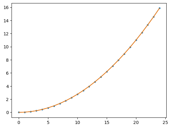
Wave height as function of wind speed
$$ H = kv^2 $$
https://planetcalc.com/4442/ uses \(k=0.0275\)
Combining everything one obtains
$$ 0.0275v^2 = 21(S/10)^{2.8} $$
and therefore
$$ v=27.6(S/10)^{1.4} $$
Turbulence
Noise due to ocean turbulences dominates the very low frequencies (<10 Hz) and may be modeled as
$$ NL_{term}(f)= 17-30\log(f) $$
with frequency \(f\) in kHz
Thermal noise
Thermal noise dominates the very high frequency spectrum (>50 kHz) and may be modeled as
$$ NL_{term}(f)= -15+20\log(f) $$
with frequency \(f\) in kHz
Develop function wind as function of sea state
To develop a relationship between sea state and wind speed one may combine the two two tables: wave height(sea state) and wind speed(wind speed)
import numpy as np
import matplotlib.pyplot as plt

# wave height as function of sea state
C=np.array(
    [[0,0],
     [1,(0+0.1)/2],
     [2,(0.1+0.5)/2],
     [3,(0.5+1.25)/2],
     [4,(1.25+2.5)/2],
     [5,(2.5+4)/2],
     [6,(4+6)/2],
     [7,(6+9)/2],
     [8,(9+14)/2],
     [9,(14+18)/2]
     ]
)
plt.plot(C[:,0],C[:,1],'.-')
plt.plot(C[:,0],21*(C[:,0]/10)**2.8,'.-')
plt.show()

# wave height as function of wind speed as used by https://planetcalc.com/4442/
D=np.array(
[[0 , 0],
 [1 , 0.03],
 [2, 0.11],
 [3 , 0.25],
 [4 , 0.44],
 [5 , 0.69],
 [6 , 0.99],
 [7 , 1.35],
 [8 , 1.76],
 [9 , 2.23],
 [10 , 2.75],
 [11, 3.33],
 [12 , 3.96],
 [13 , 4.65],
 [14 , 5.40],
 [15 , 6.19],
 [16 , 7.05],
 [17 , 7.96],
 [18 , 8.92],
 [19 , 9.94],
 [20 , 11.01],
 [21 , 12.14],
 [22 , 13.33],
 [23 , 14.56],
 [24 , 15.86]])

plt.plot(D[:,0],D[:,1],'.-')
plt.plot(D[:,0],0.0275*D[:,0]**2)
plt.show()

# final plot
plt.plot(C[:,0],np.interp(C[:,1],D[:,1],D[:,0]),'o-')
plt.plot(C[:,0],27.6*(C[:,0]/10)**1.4)
plt.show()
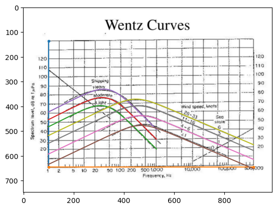
Digitizing published Wenz curves
To obtain some equations for ship and wind driven surface noise, a figure of published Wenz curves is digitized by trial and the equation constructed to fit the data and figure.
import numpy as np
import matplotlib.pyplot as plt

wenz='C:/Users/zimme/Pictures/Wenz1.png'
img =plt.imread(wenz)

def X(x): return 100+x*(915-100)/np.log10(500000)
def Y(y): return 645-y*(645-135)/140

def NL_surf(w,f):
    fo=1/(2.78+0.14*w**0.75)
    return 44+28*np.log10(1+w**0.75)+19*np.log10(f)-18*np.log10(f**2+fo**2)

def NL_ship(w,f):
    return 20+11*w+20*np.log10(f)-30*np.log10(f**2+(15+w*4)/10**4)

plt.imshow(img,aspect='auto')
plt.plot([100,100],[135,645],'.-')
plt.plot([100,915],[645,645],'.-')

ff1=np.arange(1,1000)
ff2=np.arange(1,500000)

plt.plot(X(np.log10(ff1)),Y(NL_ship(0, ff1/1000)))
plt.plot(X(np.log10(ff1)),Y(NL_ship(1, ff1/1000)))
plt.plot(X(np.log10(ff1)),Y(NL_ship(2, ff1/1000)))

plt.plot(X(np.log10(ff2)),Y(NL_surf(  0, ff2/1000)))
plt.plot(X(np.log10(ff2)),Y(NL_surf(1.5, ff2/1000)))
plt.plot(X(np.log10(ff2)),Y(NL_surf(  7, ff2/1000)))
plt.plot(X(np.log10(ff2)),Y(NL_surf( 16, ff2/1000)))

plt.show()
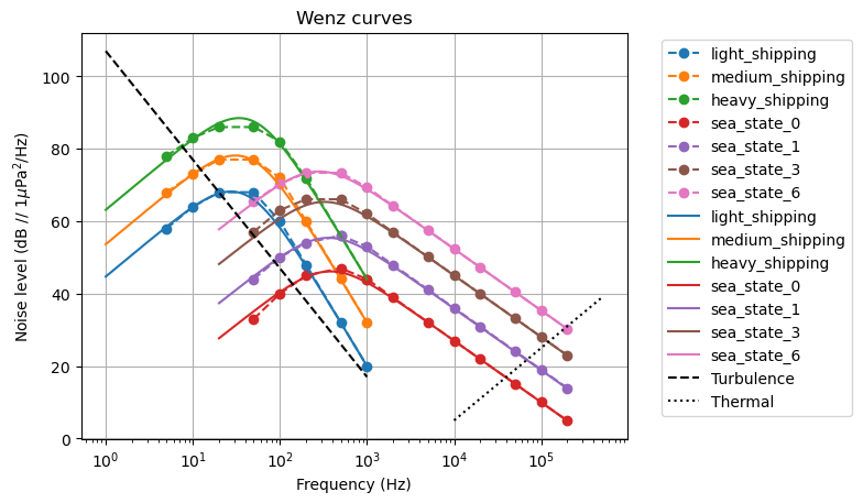
# Wenz curves

frequency_Hz=np.array([5,10,20,50,100,200,500,1000,2000,5000,10000,20000,50000,100000,200000])

light_shipping =60-np.concatenate((np.array([2,-4,-8,-8,0]), 40*np.log10(np.array([2,5,10]))))
medium_shipping=60-np.concatenate((np.array([4,-1,-5,-5,0]), 40*np.log10(np.array([2,5,10]))))+12
heavy_shipping =60-np.concatenate((np.array([6, 1,-2,-2,2]), 40*np.log10(np.array([2,5,10]))))+24

sea_state_0=44-np.concatenate((np.array([11,4,-1,-3]), 17*np.log10(np.array([1,2,5,10,20,50,100,200]))))
sea_state_1=44-np.concatenate((np.array([9, 3,-1,-3]), 17*np.log10(np.array([1,2,5,10,20,50,100,200]))))+ 30*np.log10(1+1)
sea_state_3=44-np.concatenate((np.array([5,-1,-4,-4]), 17*np.log10(np.array([1,2,5,10,20,50,100,200]))))+ 30*np.log10(1+3)
sea_state_6=44-np.concatenate((np.array([4,-1,-4,-4]), 17*np.log10(np.array([1,2,5,10,20,50,100,200]))))+ 30*np.log10(1+6)

def NL_ship(w,f):
    if type(w)==list:
        w=np.array(w).reshape(1,-1)
    if type(f)==list:
        f=np.array(f).reshape(-1,1)
    elif type(f)==np.ndarray:
        f=f.reshape(-1,1)
    fo=(15+w*4)/10**4
    return 20+12*w+20*np.log10(f)-30*np.log10(f**2+fo)

def NL_surf(w,f):
    if type(w)==list:
        w=np.array(w).reshape(1,-1)
    if type(f)==list:
        f=np.array(f).reshape(-1,1)
    elif type(f)==np.ndarray:
        f=f.reshape(-1,1)
    fo=1/(2.78+0.14*w**0.75)
    return 44+28*np.log10(1+w**0.75)+19*np.log10(f)-18*np.log10(f**2+fo**2)

def windSpeed(s):
    if type(s)==list:
        s=np.array(s).reshape(1,-1)
    return 27.6*(s/10)**1.4

ff1=np.arange(1,1000)
ff2=np.arange(20,200000)

shipping= np.vstack((light_shipping,medium_shipping,heavy_shipping)).T
shipping_labels=['light_shipping','medium_shipping','heavy_shipping']

sea_state= np.vstack((sea_state_0,sea_state_1,sea_state_3,sea_state_6)).T
sea_state_labels=['sea_state_0','sea_state_1','sea_state_3','sea_state_6']

plt.figure()
plt.semilogx(frequency_Hz[:8],shipping, 'o--', label=shipping_labels)
plt.semilogx(frequency_Hz[3:],sea_state,'o--', label=sea_state_labels)
#
plt.gca().set_prop_cycle(None)
plt.semilogx(ff1,NL_ship([0,1,2], ff1/1000),label=shipping_labels)
plt.semilogx(ff2,NL_surf(windSpeed([0,1,3,6]) , ff2/1000), label=sea_state_labels)

ff3=np.array([1,1000])
plt.semilogx(ff3,17-30*np.log10(ff3/1000),'k--', label='Turbulence')

ff4=np.array([10000,500000])
plt.semilogx(ff4,-15+20*np.log10(ff4/1000),'k:', label='Thermal')

plt.title('Wenz curves')
plt.xlabel('Frequency (Hz)')
plt.ylabel('Noise level (dB // $1\\mu$Pa$^2$/Hz)')
plt.legend(bbox_to_anchor=(1.05,1))
plt.grid(True)
plt.show()
Ambient Noise class
# ambient noise spectrum estimation using Wenz and Knudsen curves
class AmbientNoise:
    def __init__(self, freq, ship=0, seaState= None, windSpeed = None):
        self.freq=freq
        self.ship=ship
        self.seaState=seaState
        self.windSpeed=windSpeed
        #
        if type(freq)==list:
            self.freq=np.array(freq).reshape(-1,1)
        elif type(freq)== np.ndarray:
            if self.freq.ndim==1:
                self.freq=freq.reshape(-1,1)
        #
        if type(ship)==list:
            self.ship=np.array(ship).reshape(1,-1)
        if type(seaState)==list:
            self.seaState=np.array(seaState).reshape(1,-1)
        if type(windSpeed)==list:
            self.windSpeed=np.array(windSpeed).reshape(1,-1)
        #
        if self.windSpeed == None:
            if type(seaState)== list:
                self.windSpeed=self.wind_speed(self.seaState)
            elif self.seaState == None:
                self.windSpeed=0
            else:
                self.windSpeed=self.wind_speed(self.seaState)

    def NL_ship(self):
        f=self.freq
        w=self.ship
        fo=(15+w*4)/10**4
        return 20+12*w+20*np.log10(f)-30*np.log10(f**2+fo)

    def NL_surf(self):
        f=self.freq
        w=self.windSpeed
        fo=1/(2.78+0.14*w**0.75)
        return 44+28*np.log10(1+w**0.75)+ 19*np.log10(f)- 18*np.log10(f**2+fo**2)

    def wind_speed(self,s):
        return 27.6*(s/10)**1.4

    def turbulence(self):
        f=self.freq
        return 17-30*np.log10(f)

    def thermal(self):
        f=self.freq
        return -15+20*np.log10(f)

    def NL_total(self):
        ship_noise  = 10**(self.NL_ship()/10)
        sea_noise   = 10**(self.NL_surf()/10)
        turb_noise  = 10**(self.turbulence()/10)
        therm_noise = 10**(self.thermal()/10)
        return 10*np.log10(ship_noise+sea_noise+turb_noise+therm_noise)

    def simulate(self,T=1, fs=48000, nfft=1024):
        nfr=1+nfft//2
        ff= np.arange(nfr)*fs/nfft
        ff[0]=ff[1]

        NL=self.NL_total()
        nlx=np.interp(ff/1000,self.freq[:,0],NL[:,0])
        A=10**(nlx/20).reshape(-1,1)
        #
        M=T*fs//nfft
        n2 = np.random.random((nfr,M))
        p2 = 2*np.pi*n2
        d2 = A*np.exp(1j*p2)/np.sqrt(2*np.pi)
        x = np.fft.irfft(d2,axis=0)
        #
        x = x.T.reshape(-1,1)
        #
        return x,A,ff
# example usage of ambient noise model
# initialize ambient noise class
ff=np.arange(1,400000)
ffk=ff/1000
if 0:
# use default parameters
AN=AmbientNoise(ffk)
else:
# use parameter explicitely
shipDensity=[0,1,1]
seaState =[0,3,6]
AN=AmbientNoise(freq=ffk, ship=shipDensity, seaState=seaState)
# fetch noise
NL_totalNoise=AN.NL_total()
# fetch components for plotting
ship_noise=AN.NL_ship()
surf_noise=AN.NL_surf()
turbulence=AN.turbulence()
thermal =AN.thermal()
NL_components=np.hstack((ship_noise, surf_noise, turbulence, thermal))
#
shipLabels=['light','medium','heavy']
shipList=[shipLabels[i]+' shipping' for i in shipDensity]
shipStyle=['-']*len(shipDensity)
shipColor=['C'+str(i) for i in shipDensity]
seaList=['sea state '+str(i) for i in seaState]
seaStyle=['-']*len(seaState)
seaColor=['C'+str(i) for i in seaState]
NL_labels=shipList + seaList + ['Turbulence', 'Thermal']
NL_lineStyles=shipStyle+ seaStyle+['--',':']
NL_colors=shipColor+seaColor+['k','k']
# plot componants and total ambient noise
plt.figure()
plt.semilogx(ff,NL_components,label=NL_labels)
plt.semilogx(ff,NL_totalNoise,'k',linewidth=2,label='total Noise')
plt.ylim(0,120)
# adjust line styles and colors
for line, ls, col in zip(plt.gca().get_lines(), NL_lineStyles, NL_colors):
line.set_linestyle(ls)
line.set_color(col)
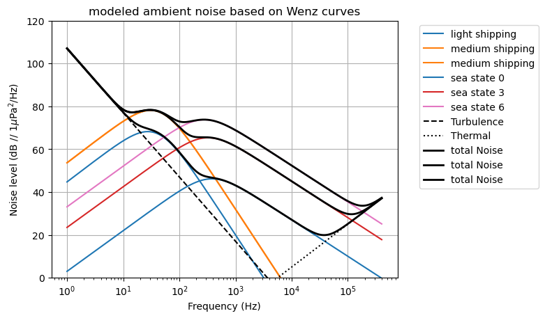
plt.title('modeled ambient noise based on Wenz curves')
plt.xlabel('Frequency (Hz)')
plt.ylabel('Noise level (dB // $1\\mu$Pa$^2$/Hz)')
plt.legend(bbox_to_anchor=(1.05,1))
plt.grid(True)
plt.show()
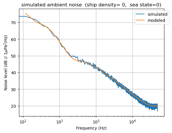
Noise simulation
Simulate ambient noise using the Wenz-Knudsen curves
import scipy.signal as signal

# initialize ambient noise model
ff=np.arange(1,400000)
ffk=ff/1000
if 0:
    # use default parameters
    AN=AmbientNoise(ffk)
else:
    # use parameter explicitely
    shipDensity=0
    seaState   =0
    AN=AmbientNoise(freq=ffk, ship=shipDensity, seaState=seaState)

# define simulation parameters
T=1             # data length (s)
nfft=8*1024     # fft size
fs=96000        # sampling frequency (Hz)
No=40           # noise level at 1 kHz

xx,A,fa=AN.simulate(T=T,fs=fs,nfft=nfft)

#convert simulated data from 1/Hz to 1/sample
xx *= (fs/2)
fx,px=signal.welch(xx,fs,nperseg=nfft,axis=0,scaling='density')

plt.figure()
plt.semilogx(fx,10*np.log10(px),label='simulated')
plt.semilogx(fa,20*np.log10(A),label='modeled')

plt.title('simulated ambient noise'+f'  (ship density= {shipDensity},'+f'  sea state={seaState})')
plt.xlabel('Frequency (Hz)')
plt.ylabel('Noise level (dB // $1\\mu$Pa$^2$/Hz)')
plt.legend(bbox_to_anchor=(1.05,1))

plt.grid(True)
plt.show()
Other-than-ambient Noise simulation
def whiteNoise(f,No):
    ''' white noise (1)'''
    return No+0*f.reshape(-1,1)

def pinkNoise(f,No):
    ''' ping noise (1/f)'''
    return No/ np.where(f==0,np.inf,np.sqrt(f)).reshape(-1,1)

def brownNoise(f,No):
    ''' brown noise (1/f**2)'''
    return 1/ np.where(f==0,np.inf,f).reshape(-1,1)

def shipNoise(f,No):
    ''' ship noise'''
    return 1/ np.maximum(0.1,f).reshape(-1,1)

def ambientNoise(f,shipping,seaState):
    ''' ambient noise'''
    ff=np.where(f==0,np.min(f[f>0]),f)
    AN=AmbientNoise(ff,ship=shipping,seaState=seaState)
    return 10**(AN.NL_total()/20)

def genNoise(T,N,fs,method=whiteNoise,NL=0,shipping=0, seaState=0):
    '''
    generate colored noise
    Input:
    T       : number of seconds
    N       : number of samples per FFT
    fs      : sampling frequency
    method  : noise color method
                whiteNoise
                pinkNoise
                brownNoise
                shipNoise
                ambientNoise
    NL      : noise level at 1 kHz
    shipping: shipping density (0,1,2)
    seaState: sea state (0 - 9)

    Output:
    x: time series
    A: modeled amplitiude spectrum
    f: frequencies
    '''
    N2 = N//2+1
    f = np.arange(0,N2)*fs/N
    fk=f/1000 # kHz
    if method==ambientNoise:
        A=ambientNoise(fk,shipping,seaState)
    else:
        A = method(fk,10**(NL/20))
    #
    M=T*fs//N
    x=np.zeros((N,M))
    n2 = np.random.random((N2,M))
    p2 = 2*np.pi*n2
    d2 = A*np.exp(1j*p2)/np.sqrt(2*np.pi)
    x = np.fft.irfft(d2,axis=0)
    #
    return x.T.reshape(-1,1),A,f

import scipy.signal as signal

T=10         # data length (s)
N=8*1024    # fft size
fs=96000    # sampling frequency (Hz)
No=40       # noise level at 1 kHz

method=ambientNoise
xx,Ax,fx= genNoise(T,N,fs,method=method)

#convert simulated data from 1/Hz to 1/sample
xx *= (fs/2)

fx,px=signal.welch(xx,fs,nperseg=N,axis=0,scaling='density')

plt.figure()
plt.semilogx(fx,10*np.log10(px),label='simulated')
plt.semilogx(fx,20*np.log10(Ax),label='modeled')

plt.title('simulated noise')
plt.xlabel('Frequency (Hz)')
plt.ylabel('Noise level (dB // $1\\mu$Pa$^2$/Hz)')
plt.legend(bbox_to_anchor=(1.05,1))

plt.grid(True)
plt.show()

Lascia un commento