The Goertzel algorithm efficiently computes the discrete Fourier transform (DFT) for a limited set of frequencies. Unlike the traditional DFT, which involves multiplying each sample by a complex number and summing the results, the Goertzel algorithm utilizes real-valued coefficients (the cosine of the target frequency) and includes one additional addition operation. The complex spectrum is calculated only once at the final step.

Derivation

The derivation of the algorithm follows https://wirelesspi.com/goertzel-algorithm-evaluating-dft-without-dft/

DFT

\begin{equation} X[k]=\sum_{n=0}^{N-1}x[n]e^{-2\pi i (k/N) n} \end{equation}

multiply both sides with \(e^{2\pi i (k_0/N) N} \)

\begin{equation} X[k_0]e^{2\pi i (k_0/N) N}=\sum_{n=0}^{N-1}x[n]e^{2\pi i (k_0/N) N}e^{-2\pi i (k/N) n} \end{equation}

with \( e^{2\pi i k_0}=1 \)

\begin{equation} X[k_0]=\sum_{n=0}^{N-1}x[n]e^{2\pi i (k_0/N) (N-n)} \end{equation}

explicit

\begin{equation} X[k_0]=x[0]e^{2\pi i (k_0/N) (N-0)} +x[1]e^{2\pi i (k_0/N) (N-1)} + \cdots + x[N-1]e^{2\pi i (k_0/N) (N-N+1)} \end{equation}

which has the form of a convolution where \(x[0]\) is multiplied \(N\) times, \(x[1]\) is multiplied \(N-1\) times, and finally \(X[N-1]\) is 1 time with \(e^{2\pi i (k_0/N)}\)

Recursion

This means, that the DFT can be rewitten as

\begin{equation} X[k_0]=\Big[\cdots\Big[\Big[[x[0]e^{2\pi i (k_0/N)} +x[1]\Big]e^{2\pi i (k_0/N)} +x[2]\Big]e^{2\pi i (k_0/N)} \cdots + x[N-1]\Big]e^{2\pi i (k_0/N))} \end{equation}

which leads to the following recursion

\begin{equation} \begin{matrix} y[0]=& x[0] \\ y[1]=& y[0]e^{2\pi i (k_0/N)}+x[1]\\ y[2]=& y[1]e^{2\pi i (k_0/N)}+x[2]\\ \vdots & \end{matrix} \end{equation}

or in general

\begin{equation} y[n]= y[n-1]e^{2\pi i (k_0/N)}+x[n] \end{equation}

Z-transform

\begin{equation} Y[z]=z^{-1}Y[z]e^{2\pi i (k_0/N)} + X[z] \end{equation} that is

\begin{equation} \frac{Y[z]}{X[z]}=\frac{1}{1-z^{-1}e^{2\pi i (k_0/N)}} \end{equation}

making the denominator real

\begin{equation} \frac{Y[z]}{X[z]}=(1-z^{-1}e^{-2\pi i (k_0/N)}) \frac{1}{(1-z^{-1}e^{2\pi i (k_0/N)})(1-z^{-1}e^{-2\pi i (k_0/N)})} \end{equation}

The right-hand side is the product of two terms, allowing us to introduce on the left-hand side \(V[z]\) such that

$$ \frac{Y[z]}{X[z]}=\frac{Y[z]}{S[z]}\frac{S[z]}{X[z]} $$

and therefore

$$ \frac{Y[z]}{S[z]}=(1-z^{-1}e^{-2\pi i (k_0/N)}) $$ and $$ \frac{S[z]}{X[z]}=\frac{1}{(1-z^{-1}e^{2\pi i (k_0/N)})(1-z^{-1}e^{-2\pi i (k_0/N)})} $$ or $$ \frac{S[z]}{X[z]}=\frac{1}{1-2\cos(2\pi (k_0/N))z^{-1}+z^{-2}} $$

Algorithm

Let \(\omega_0=2\pi (k_0/N)\) we get two equations

\begin{equation} y[n]=s[n]-\exp(-i\omega_o)s[n-1] \end{equation}

\begin{equation} s[n]=x[n]+2\cos(\omega_0)s[n-1]-s[n-2] \end{equation}

for last step \(n=N\)

\begin{equation} y[N]=s[N]-\exp(-i\omega_o)s[N-1] \end{equation}

\begin{equation} s[N]=2\cos(\omega_0)s[N-1]-s[N-2] \end{equation}

combining these two equations

\begin{equation} y[N]=(\exp(i\omega_o)+\exp(-i\omega_o))s[N-1]-s[N-2]-\exp(-i\omega_o)s[N-1] \end{equation}

one gets

\begin{equation} y[N]=\exp(i\omega_o)s[N-1]-s[N-2] \end{equation}

Note

there is no need to estimate \(y[n]\), only \(y[N]\) needs to be estimated at the end of the iteration.

Also, the sign of the exponential may be negative so that imag coincides with numpy implementation of rFFT

Python code

import numpy as np
import matplotlib.pyplot as plt
from numba import  njit

@njit(cache=True)
def goertzel(xx,fx):
    n1=xx.shape[0]
    ee=np.exp(-1j*2*np.pi*fx)
    c1=2*ee.real
    s1=0*c1
    s2=0*c1
    for ii in range(n1,0,-1):
        so=xx[ii]+c1*s1-s2
        s2=s1
        s1=so
    y=xx[0]+ee*s1-s2
    return y*2/n1
#

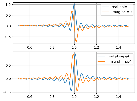
Example

fs=48000
fo=4000
fr=np.arange(0.5,1.5,0.005)
fx=fr*fo/fs

te=0.005
tt=np.arange(0,te,1/fs)
xx=np.array([np.cos(2*np.pi*fo*tt),
             np.cos(2*np.pi*fo*tt+np.pi/4)]).T
print(xx.shape)
#
yy=np.zeros((len(fr),xx.shape[1]),dtype='complex')
for ii in range(yy.shape[1]):
    yy[:,ii]=goertzel(xx[:,ii],fx)
#
plt.subplot(211)
plt.plot(fr,yy[:,0].real,label='real phi=0')
plt.plot(fr,yy[:,0].imag,label='imag phi=0')
plt.legend()
plt.grid(True)
plt.subplot(212)
plt.plot(fr,yy[:,1].real,label='real phi=pi/4')
plt.plot(fr,yy[:,1].imag,label='imag phi=pi/4')
plt.legend()
plt.grid(True)
plt.show()

if 0:
    plt.plot(tt,xx,label='signal')
    plt.plot(tt,0*tt+yy.real,label='real')
    plt.plot(tt,0*tt+yy.imag,label='imag')
    plt.legend()
    plt.grid(True)
    plt.show()

(240, 2)

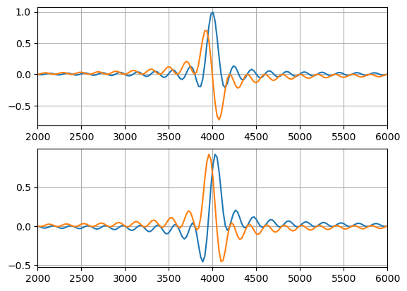
and

zz=np.fft.rfft(xx,axis=0,n=2048)
zz *=2/len(xx)
ff=np.arange(len(zz))/len(zz)*fs/2
#
plt.subplot(211)
plt.plot(ff,zz[:,0].real)
plt.plot(ff,zz[:,0].imag)
plt.xlim(0.5*fo,1.5*fo)
plt.grid(True)
plt.subplot(212)
plt.plot(ff,zz[:,1].real)
plt.plot(ff,zz[:,1].imag)
plt.xlim(0.5*fo,1.5*fo)
plt.grid(True)
plt.show()