The second article in the Multi-phone Processing series explores the technique of direction finding for sound sources. Direction finding becomes the preferred approach when localization is impractical, such as when the sound source is located at a significant distance from the hydrophone array. In this context, “significant distance” typically refers to a distance that is at least 10 times the size of the array, which is commonly the case for compact hydrophone arrays.

Direction finding

Given

\begin{equation}(h_i-h_j)^Ts=\frac{|h_i|^2-|h_j|^2-(\delta R_{ij})^2}{2}-(\delta R_{ij})R_j\end{equation}

and assuming that all phones are closely spaced compared to distance to source

and noting that

\begin{equation}(h_i-h_j)^Ts=|h_i-h_j||s|\cos{(\beta)}\end{equation}

or equivalently with \(s=|s|\hat{s}\) and dividing by \(|s|\)

\begin{equation}(h_i-h_j)^T\hat{s}=|h_i-h_j|\cos{(\beta)}\end{equation}

then

\begin{equation}|h_i-h_j|\cos{(\beta)}=\frac{|h_i|^2-|h_j|^2-(\delta R_{ij})^2}{2|s|}-(\delta R_{ij})\frac{R_j}{|s|}\end{equation}

Let

\begin{equation}R_j=|s-h_j|\end{equation}

then

\begin{equation}|h_i-h_j|\cos{(\beta)}=\frac{|h_i|^2-|h_j|^2-(\delta R_{ij})^2}{2|s|}-(\delta R_{ij})\frac{|s-h_j|}{|s|}\end{equation}

which for \(|s| \to \infty\) becomes an equation that may be used to estimate the direction \(\beta\) to a distant sound source.

\begin{equation}(h_i-h_j)^T\hat{s}=-(\delta R_{ij})\end{equation}

This equation is the basis for all direction finding algorithms that are based on time-delay of arrival (TDOA)

Multi-phone direction finding

Let

\begin{equation}(h_i-h_j)^T\hat{s}=-(\delta R_{ij})\end{equation}

and assume an array of \(n+1\) phones then one can form  \(npp=(n+1)n/2\) different pairs of phones resulting to a system of \(npp\) equations

\begin{equation}\left(\begin{matrix} (x_1-x_0)&(y_1-y_0)&(z_1-z_0)\\                        (x_1-x_0)&(y_1-y_0)&(z_1-z_0)\\                        \vdots&\vdots&\vdots\\                        (x_n-x_{n-1})&(y_n-y_{n-1})&(z_n-z_{n-1})  \end{matrix}\right)\hat{s}=-\left(\begin{matrix} \delta R_{10}\\\delta R_{20}\\\vdots\\\delta R_{n(n-1)}                        \end{matrix}\right)                        \end{equation}

With

\begin{equation}A=\left(\begin{matrix} (x_1-x_0)&(y_1-y_0)&(z_1-z_0)\\                        (x_1-x_0)&(y_1-y_0)&(z_1-z_0)\\                        \vdots&\vdots&\vdots\\                        (x_n-x_{n-1})&(y_n-y_{n-1})&(z_n-z_{n-1})  \end{matrix}\right)           \end{equation}

\begin{equation}b_1=\left(\begin{matrix} \delta R_{10}\\\delta R_{20}\\\vdots\\\delta R_{n(n-1)}                        \end{matrix}\right)  \end{equation}

the solution for the source direction vector \(\hat{s}\) becomes

\begin{equation}\hat{s}=-A^+b_1\end{equation}

It should be noted that the path difference \(\delta R_{ij}=R_i-R_j\), where \(R_j\) is the path to the reference phone, is negative if the sound arrives first to phone at \(h_i\) and then to the one at \(h_j\), as it would for \(\cos{\beta}>0\).

Four-phone direction finding

The four phones are assumed to bo not in the same plane, i.e. they are distributed in 3D.

import numpy as np
import matplotlib.pyplot as plt
#
def cosd(x): return np.cos(x*np.pi/180)
def sind(x): return np.sin(x*np.pi/180)
def tand(x): return np.tan(x*np.pi/180)

def atan2d(x,y): return np.arctan2(x,y)*180/np.pi

def direction(az,el): return np.array([cosd(az)*cosd(el),sind(az)*cosd(el),sind(el)])

#geometry
if 1:   # pyramide
    h=np.array([[0,0,0],
                [cosd(60), sind(60), 0],
                [cosd(120),sind(120),0],
                [0,sind(60)-tand(30)/2, np.sqrt(1-(sind(60)-tand(30)/2)**2)]])
else:   # on cube
    h=np.array([[ 1,-1,-1],
                [-1, 1,-1],
                [-1,-1, 1],
                [ 1, 1, 1]])/(2*np.sqrt(2))

#estmate hydrophone connection vectors
dsel=np.array([[1,0],[2,0],[3,0],[2,1],[3,1],[3,2]])
im1=dsel[:,0]
im0=dsel[:,1]
D=h[im1,:]-h[im0,:]
L=np.sqrt(np.sum(D**2,1))
#
#print(h)
#print(L)

# invert geometry needed for direction finding
DI=np.linalg.pinv(D)
print(DI.shape)
print(np.linalg.matrix_rank(DI))

(3, 6)
3

# simulated direction
az=45
el=30

S=direction(az,el)

# simulate path differences
DR=-np.sum(D*S,1)
print(DR)

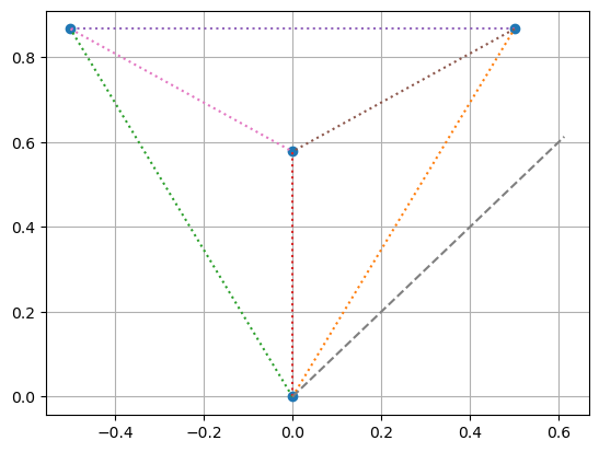
plt.plot(h[:,0],h[:,1],'o')
plt.plot(h[[0,1],0],h[[0,1],1],':')
plt.plot(h[[0,2],0],h[[0,2],1],':')
plt.plot(h[[0,3],0],h[[0,3],1],':')
plt.plot(h[[1,2],0],h[[1,2],1],':')
plt.plot(h[[1,3],0],h[[1,3],1],':')
plt.plot(h[[2,3],0],h[[2,3],1],':')
plt.plot([0,S[0]],[0,S[1]],'--')
plt.grid(True)
plt.show()

[-0.8365163  -0.22414387 -0.76180168  0.61237244  0.07471462 -0.53765781]

def directionFinding(DI,M):
    #direction finding
    SX=-DI@M

    # estimate and print angles
    az=np.arctan2(SX[1],SX[0])*180/np.pi
    el=np.arctan2(SX[2],np.sqrt(SX[0]**2+SX[1]**2))*180/np.pi
    return az,el

az,el=directionFinding(DI,DR)
print(az,el)

45.00000000000001 30.000000000000004

Three-phone direction finding

With three phones, the matrix \(A^+\) is not of full rank but, being minimum norm, the result can be extended to a full solution. However, this can only be done if the vector norm of the source direction is known. Typically, if the sound speed is known then the source direction vector norm is also known and this method can be applied.

Let the 3-phone estimation of source direction vector \(\hat{s}_2\) be

\begin{equation}\hat{s}_2=-A^+b_1\end{equation}

then the final (3-D) source direction vector \(\hat{s}[latex] may be estimated via

\begin{equation}\hat{s}=\hat{s}_2 \pm \hat{N} \sqrt{1-|\hat{s}_2|^2}\end{equation}

where

$$ \hat{N}=\frac{A^+_0 \times A^+_1}{|A^+_0 \times A^+_1|}$$

with [latex]A^+_i\) denoting the i-th column vector of \(A^+\).

To extend \(\hat{s}_2\) to \(\hat{s}\), a direction vector \(\hat{N}\) is estimated that is perpendicular to the 3-phone plain and multiplied with the ‘missing’ vector norm of the direction vector  \(\hat{s}\).

As each plain has a up-down ambiguity, the sign of the correction must be selected accordingly, that is, the expected source vector \(S_e\) should be on the same side of the  direction vector \(\hat{N}\), or  \((\hat{N}^T S_e>0)\).

import numpy as np
import matplotlib.pyplot as plt
#
#geometry
# select sub array
hsel=[0,1,3]
h1=h[hsel,:]

#estmate hydrophone connection vectors
dsel=np.array([[1,0],[2,0],[2,1]])
im1=dsel[:,0]
im0=dsel[:,1]
D=h1[im1,:]-h1[im0,:]

# invert geometry needed for direction finding
DI=np.linalg.pinv(D)
print(DI.shape)
print(np.linalg.matrix_rank(DI))

(3, 3)
2

# simulated direction
az=130
el=-30

S=direction(az,el)

# simulate path differences (project hydrophone differences onto source direction)
DR=-np.sum(D*S,1)

def directionFinding(DI,M,sign=+1):
    #direction finding
    SX=-DI@M

    #correct for 3-phine estimation
    if np.linalg.matrix_rank(DI)==2:
        Nx = sign*np.cross(DI[:,0],DI[:,1])
        Nx /= np.linalg.norm(Nx,2)
        SX += Nx*np.sqrt(1-(SX**2).sum())

    # estimate and return angles
    az=np.arctan2(SX[1],SX[0])*180/np.pi
    el=np.arctan2(SX[2],np.sqrt(SX[0]**2+SX[1]**2))*180/np.pi
    return az,el,Nx

az,el,Nx=directionFinding(DI,DR)
if Nx@S<0:
    az,el,Nx=directionFinding(DI,DR,-1)
print(az,el,Nx@S>0)

130.00000000000003 -29.999999999999986 True