The third article on multi-phone processing addresses beamforming, which is a technique that is different to multi-phone localization or multi-phone direction finding. Both methods (localization and direction finding) require first the detection of signals and then allow the signal processing. Beamforming can be considered as spatial filters that maximizes the response (beamformer output) for any selected look direction.
Beam forming
Beamforming is also based on the fact that signal (here sound) arrives at different times at distributed (array of) sensors (here hydrophones).
While the direction of single sound source may be estimated by measuring the relative delays within the hydrophone array and relating these measurements to the array geometry, beamforming analyses the arriving sound field for all possible directions (beams).
Basic formulation
Let the sound pressure measured an a single hydrophone be composed of a signal \(s\) and some noise \(n\)
\begin{equation}x(t)=s(t)+n(t)\end{equation}
then in an array of hydrophones the measurements become
\begin{equation}x_i(t)=s(t-\tau_i(\alpha,\beta))+n(t)\end{equation}
where \(\tau_i(\alpha,\beta)\) is the delay of the signal at hydrophone \(i\) with respect to some reference hydrophone and \(\alpha,\beta\) are the angles of arrival
For a line array with equally spaced hydrophones the delay has a simple form
\begin{equation}\tau_i(t)=i\frac{d}{c}\cos{\gamma}\end{equation}
where \(d\) id the hydrophone spacing, \(c\) is the sound speed at the hydrophone, and \(\gamma\) is the relative angle of arrival, that for a line array is composed of the azimuth \(\alpha\) and elevation angle \(\beta\).
\begin{equation}\cos{\gamma}=\cos{\alpha}\cos{\beta}\end{equation}
The beamforming algorithm simply speaking tries to undo the signal delays \(\tau_i(\alpha,\beta)\) by compensating with negative delays
\begin{equation}x(t)=\frac{1}{N}\sum_i (x_i(t+\delta_i(\gamma)))\end{equation}
In cases, where \(\delta_i(\gamma)=\tau_i(\alpha,\beta)\) we get
\begin{equation}x(t)=s(t)+\frac{1}{N}\sum_i(n(t+\delta_i(\gamma)))\end{equation}
indicating that the signal \(s(t)\) is completely reconstructed and that noise, that is assumed to be uncorrelated is attenuated by the summing of the amplitudes.
All other signals that do not correspond to the assumed delays are also attenuated due to delay mismatch.
Delay estimation
This operation is related to the simulation of measurements using azimuth and elevation angles.
In particular, given a source direction \(s\) that is obtained from azimuth and elevation angles and therefore
\begin{equation}(h_i-h_j)^T\hat{s}=(\delta R_{ij})\end{equation}
then the number of fractional samples \(\delta N_{ij}\) that is needed to align the arriving time series is estimated by
\begin{equation}\delta N_{ij}=\frac{f_s}{c}(h_i-h_j)^T\hat{s}\end{equation}
where \(f_s\) is the sampling frequency, \(c\) is the sound speed.
Beam steering
A general application of beamforming, where the signal direction is unknown, will vary the steering vector \(s\) to cover all possible directions resulting in \(N_\alpha \times N_\beta\) directions, where \(N_\alpha, N_\beta\) are the numbers of different azimuth and elevation directions.
Beam forming does not require knowledge on the source location, but combines the array data in such a way that the look direction (or beam) is steered across the angles of interest. Signals, that coincide with the steering direction are maintained and noise or other signals, that are in different directions are attenuated.
Simulation
In the following we simulate the beamforming with a line array of Cuvier’s beaked whale (Zc) clicks
## Simulation of Zc clicks
import numpy as np
import matplotlib.pyplot as plt

def zcSig(tt,f0,fm,aa,bb,cc):
    return (aa*tt)**bb * np.exp(-(aa*tt)**cc + 2*np.pi*1j*(f0+fm*tt)*tt)

fs=192 #kHz
ts=1 #ms
tt=np.arange(0,ts,1/fs)

f0=30
fm=60
aa=13
bb=1.5
cc=1.5
ss=zcSig(tt,f0,fm,aa,bb,cc)
ss=np.append(np.zeros((20,1)),ss)
tt=(-20+np.arange(len(ss)))/fs
#tt=np.arange(-20/fs,ts,1/fs)

plt.plot(tt,np.real(ss));
plt.plot(tt,np.abs(ss));
plt.grid(True)
plt.show()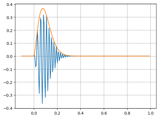
Line array
A line array of hydrophones is modelled having a ‘design frequency’ of 60 kHz. that is \(\lambda/2=1.25\) cm. This is rather close for real hydrophones, but would allow beamforming of Zc clicks.
# Line array
c=1500      # m/s sound speed
d=0.0125    # hydrophone spacing (0.75/60)
N=10        # number of hydrophones
h=np.arange(N)*d
Filter utility
The following code is a convenience function that allows multi-channel FFT based FIR filter.
#
# Overlap-add FIR filter, (c) Joachim Thiemann 2016
# https://github.com/jthiem/overlapadd/blob/master/olafilt.py
#
def fftfilt(b, x, zi=None):
    """
    Filter a one-dimensional array with an FIR filter

    Filter a data sequence, `x`, using a FIR filter given in `b`.
    Filtering uses the overlap-add method converting both `x` and `b`
    into frequency domain first.  The FFT size is determined as the
    next higher power of 2 of twice the length of `b`.

    Parameters
    ----------
    b : one-dimensional numpy array
        The impulse response of the filter
    x : one-dimensional numpy array
        Signal to be filtered
    zi : one-dimensional numpy array, optional
        Initial condition of the filter, but in reality just the
        runout of the previous computation.  If `zi` is None or not
        given, then zero initial state is assumed.

    Returns
    -------
    y : array
        The output of the digital filter.
    zf : array, optional
        If `zi` is None, this is not returned, otherwise, `zf` holds the
        final filter delay values.
    """

    L_I = b.shape[0]
    # Find power of 2 larger that 2*L_I (from abarnert on Stackoverflow)
    L_F = 2<<(L_I-1).bit_length()
    L_S = L_F - L_I + 1
    L_sig = x.shape[0]
    offsets = range(0, L_sig, L_S)

    # handle complex or real input
    if np.iscomplexobj(b) or np.iscomplexobj(x):
        fft_func = np.fft.fft
        ifft_func = np.fft.ifft
        res = np.zeros(L_sig+L_F, dtype=np.complex128)
    else:
        fft_func = np.fft.rfft
        ifft_func = np.fft.irfft
        res = np.zeros(L_sig+L_F)

    FDir = fft_func(b, n=L_F)

    # overlap and add
    for n in offsets:
        res[n:n+L_F] += ifft_func(fft_func(x[n:n+L_S], n=L_F)*FDir)

    if zi is not None:
        res[:zi.shape[0]] = res[:zi.shape[0]] + zi
        return res[:L_sig], res[L_sig:]
    else:
        return res[:L_sig]
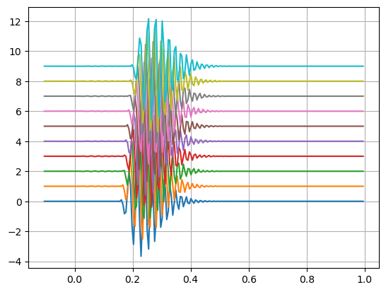
Simulate measurements
– estimate the arrival times (up to a constant) for all hydrophones
– delay time series using a fractional sinc function
A sinc function is used as it is an all-pass filter with well defined delay properties. Other interpolating low-pass filter may be used (e.g. Kaiser filters). The filters should be of FIR type to have well defined delay properties.
Here, to simplify the algorithm, no integer resampling is done, requiring somewhat more coefficients to minimize edge effects.
# measurements
import scipy.signal as signal

fs=192000
#
if 0:
    # noise
    noise_power = 0.001 * fs / 2
    ndat=fs//100
    M=np.random.normal(scale=np.sqrt(noise_power), size=(N,ndat))

    # estimate power spectral density (PSD)
    win=signal.get_window("hann",1024)
    f, Pxx_dens = signal.welch(M[0,:], fs=fs, nperseg=len(win), noverlap=0, scaling="density", window=win)

    plt.semilogy(f/1000, Pxx_dens)
    plt.xlabel('Frequency [kHz]')
    plt.ylabel('PSD [V**2/Hz]')
    plt.ylim(1e-6,1e-1)
    plt.grid(True)

    plt.show()

# signal
iao=60  # simulated angle

xo=ss.real
# simulated delays relative to hydrophone 0
tau=np.arange(N)*d/c*np.cos(iao*np.pi/180)

yy=np.zeros((len(xo),N))

kk=np.arange(-30,30,1);
for ii in range(N):
    uu=np.sinc(kk-tau[ii]*fs)
    yy[:,ii]=fftfilt(uu,xo)

plt.plot(tt,yy*10+np.ones((yy.shape[0],1))*range(N))
plt.grid(True)
plt.show()
Check steering
To check the method, compensate the simulated delays so that all hydrophone receive the signal in parallel.
# check steering (replace sinc(kk-tau[ii]*fs) by sinc(kk+tau[ii]*fs))
vv=np.zeros((len(ss),N))
for ii in range(N):
    uu=np.sinc(kk+tau[ii]*fs)
    vv[:,ii]=fftfilt(uu,yy[:,ii])
plt.plot(tt,vv*10+np.ones((vv.shape[0],1))*range(N))
plt.grid(True)
plt.show()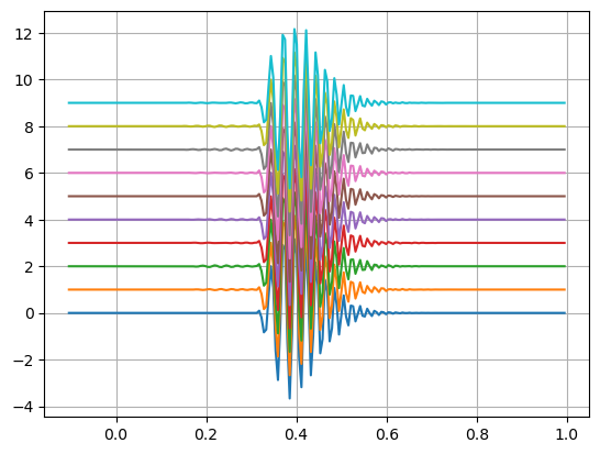
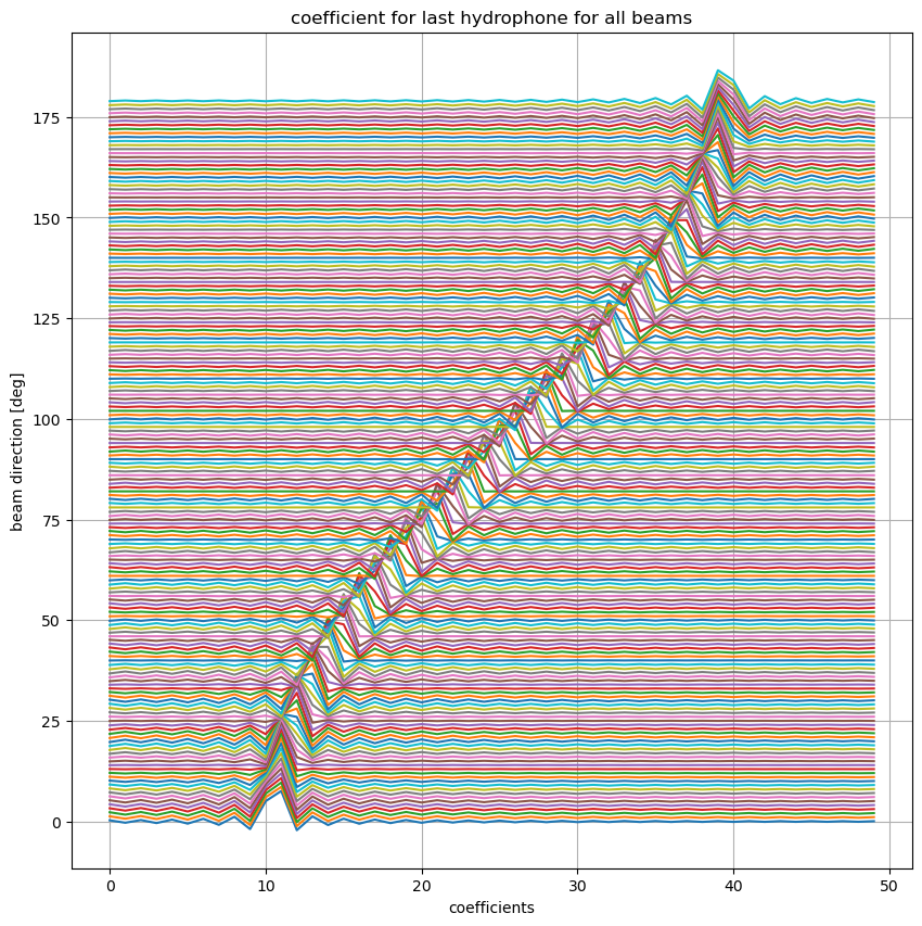
Spatial filter (beam forming)
Here the complete beamformer is presented.
– Create first the filter coefficient matrix
– filter all hydrophone using the adequate coefficients.
– for each time step average all hydrophones
An inspection of the coefficients indicate that for the 0 and 180 deg cases edge effects may occur at the end of the array.
# beamformer

def delayMatrix(dd,maxDel):
    # generate delay coefficient matrix
    nc=np.ceil(maxDel)+10  # assume nimimum sinc coefficients: -10:10
    kk=np.arange(-nc,nc)
    #
    ww = np.zeros((len(kk),dd.shape[0],dd.shape[1]))
    for cc in range(ndir):              # over all beams
        for ii in range(N):             # over all hydrophones
            arg=kk+dd[ii,cc]
            ww[:,ii,cc]=np.sinc(arg)
    return ww


ndir=180
dd=h.reshape(-1,1)/c*np.cos(np.arange(ndir)/ndir*np.pi)*fs
maxDel=h[-1]/c*fs
ww=delayMatrix(dd,maxDel)

plt.figure(figsize=(10,10))
plt.title('coefficient for last hydrophone for all beams')
plt.plot(ww[:,-1,:]*10+np.ones((ww.shape[0],1))*range(ndir))
plt.xlabel('coefficients')
plt.ylabel('beam direction [deg]')
plt.grid(True)
plt.show()
# filter data (beamformer)
def beamform(ww,yy):
vv=np.zeros(yy.shape)
zz=np.zeros((yy.shape[0],ww.shape[2]))
for cc in range(ndir): # over all beams
for ii in range(N): # over all hydrophones
vv[:,ii]=fftfilt(ww[:,ii,cc],yy[:,ii])
zz[:,cc]=np.mean(vv,axis=1) # sum hydrophones for each beam
return zz
#
zz=beamform(ww,yy)
#
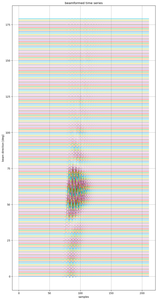
# visualize beamformer response as waterfall plot
plt.figure(figsize=(10,20))
plt.title('beamformed time series')
plt.plot(zz*10+np.ones((zz.shape[0],1))*range(ndir))
plt.xlabel('samples')
plt.ylabel('beam direction [deg]')
plt.grid(True)
plt.show()
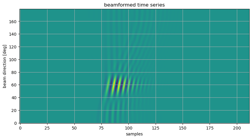
# visualize beamformer response as image (color-code amplitude)
plt.figure(figsize=(10,5))
plt.title('beamformed time series')
plt.imshow(zz.T,aspect='auto',origin='lower')
plt.xlabel('samples')
plt.ylabel('beam direction [deg]')
plt.grid(True)
plt.show()
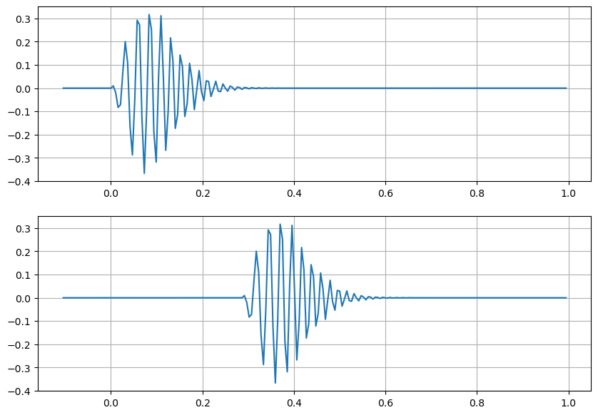
#
# compare with input signal at best steering
plt.figure(figsize=(10,7))
plt.subplot(211)
plt.plot(tt,ss.real)
plt.grid(True)
plt.subplot(212)
plt.plot(tt,zz[:,iao])
plt.grid(True)
plt.show()
Lascia un commento